Note
This tech note is a collection of Qserv prototyping experiments drawn from different locations. The first two sections were originally published in [4] and subsequently [9] (see DocuShare version 18). Document LDM-135 no longer contains the historical background and the content has been migrated to different locations. The later sections are tests from LSST Trac that were referenced from the first two sections of LDM-135.
1 Design Trade-Offs¶
The LSST database design involves many architectural choices. Example of architectural decisions we faced include how to partition the tables, how many levels of partitioning is needed, where to use an index, how to normalize the tables, or how to support joins of the largest tables. This chapter covers the test we run to determine the optimal architecture of MySQL-based system.
1.1 Standalone Tests¶
1.1.1 Spatial join performance¶
This test was run to determine how quickly we can do a spatial self-join
(find objects within certain spatial distance of other objects) inside a
single table. Ultimately, in our architecture, a single table represents
a single partition (or sup-partition). The test involved trying various
options and optimizations such as using different indexes (clustered and
non clustered), precalculating various values (like COS(RADIANS(decl))),
and reordering predicates. We run these tests for all reasonable table
sizes (using MySQL and PostgreSQL). We measured CPU and disk I/O to
estimate impact on hardware. In addition, we re-run these tests on the
lsst10 machine at NCSA to understand what performance we may expect
there for DC3b [11]. These tests are documented below.
We found that
PostgreSQL was 3.7x slower for spatial joins over a range of row counts,
and reducing the row-count per partition to less than 5k rows was
crucial in achieving lowering compute intensity, but that predicate
selectivity could compensate for a 2-4x greater row count.
1.1.2 Building sub-partitions¶
Based on the “spatial join performance” test we determined that in order to speed up self-joins within individual tables (partitions), these partitions need to be very small, \(O(\mathrm{few~} K)\) rows. However, if we partition large tables into a very large number of small tables, this will result in unmanageable number of tables (files). So, we determined we need a second level of partitioning, which we call sub-partition on the fly. This test included:
- sub-partitioning through queries:
- one query to generate one sub-partition
- relying on specially introduced column (
subPartitionId).
- segregating data into sub-partitions in a client C++ program, including using a binary protocol.
We timed these tests. This test is described below. These tests showed that it was fastest to build the on-the-fly sub-partitions using SQL in the engine, rather than performing the task externally and loading the sub-partitions back into the engine.
1.1.3 Sub-partition overhead¶
We also run detailed tests to determine overhead of introducing
sub-partitions. For this test we used a 1 million row table, measured
cost of a full table scan of such table, and compared it against
scanning through a corresponding data set partitioned into
sub-partitioned. The tests involved comparing in-memory with
disk-based tables. We also tested the influence of introducing
“skinny” tables, as well as running sub-partitioning in a client C++
program, and inside a stored procedure. These tests are described at
below. The on-the-fly
overhead was measured to be 18% for select * queries, but
3600% if only one column (the skinniest selection) was needed.
1.1.4 Avoiding materializing sub-partitions¶
We tried to run near neighbor query on a 1 million row table. A starting point is 1000 sec which is ~16 min 40 sec (based on earlier tests we determined it takes 1 sec to do near neighbor for 1K row table).
The testing included:
- Running near neighbor query by selecting rows with given subChunkId into in memory table and running near neighbor query there. It took 7 min 43 sec.
- Running near neighbor query by running neighbor once for each subChunkId, without building sub-chunks. It took 39 min 29 sec.
- Running near neighbor query by mini-near neighbor once for each subChunkId, without building sub-chunks, using in-memory table. It took 13 min 13 sec.
1.1.5 Billion row table / reference catalog¶
One of the catalogs we will need to support is the reference catalog, even in DC3b it is expected to contain about one billion rows. We have run tests with a table containing 1 billion rows catalog (containing USNO-B data) to determine how feasible it is to manage a billion row table without partitioning it. These tests are described in detail below. This revealed that single 1-billion row table usage is adequate in loading and indexing, but query performance was only acceptable when the query predicates selectivity using an index was a small absolute number of rows (1% selectivity is too loose). Thus a large fraction of index-scans were unacceptably slow and the table join speed was also slow.
1.1.6 Compression¶
We have done extensive tests to determine whether it is cost effective to compress LSST databases. This included measuring how different data types and indexes compress, and performance of compressing and decompressing data. These tests are described in details below. We found that table data compressed only 50%, but since indexes were not compressed, there was only about 20% space savings. Table scans are significantly slower due to CPU expense, but short, indexed queries were only impacted 40-50%.
1.1.7 Full table scan performance¶
To determine performance of full table scan, we measured:
- raw disk speed with
dd if=<large file> of=/dev/zeroand got 54.7 MB/sec (2,048,000,000 bytes read in 35.71 sec) - speed of
select count(*) from XX where muRA = 4.3using a 1 billion row table. There was no index on muRA, so this forced a full table scan. Note that we did not doSELECT *to avoid measuring speed of converting attributes. The scan of 72,117,127,716 bytes took 28:49.82 sec, which is 39.8 MB/sec.
So, based on this test the full table scan can be done at 73% of the raw disk speed (using MySQL MyISAM).
1.1.8 Low-volume queries¶
A typical low-volume queries to the best of our knowledge can be divided into two types:
analysis of a single object. This typically involves locating a small number of objects (typically just one) with given objectIds, for example find object with given id, select attributes of a given galaxy, extract time series for a given star, or select variable objects near known galaxy. Corresponding representative queries:
SELECT * from Object where objectId=<xx>
SELECT * from Source where objectId =<xx>
analysis of objects meeting certain criteria in a small spatial region. This can be represented by a query that selects objects in a given small ra/dec bounding box, so e.g.:
SELECT * FROM Object
WHERE ra BETWEEN :raMin AND :raMax
AND decl BETWEEN :declMin AND :declMax
AND zMag BETWEEN :zMin AND :zMax
Each such query will typically touch one or a few partitions (few if the needed area is near partition edge). In this test we measured speed for a single partition.
Proposed partitioning scheme will involve partitioning each large table into a “reasonable” number of partitions, typically measured in low tens of thousands. Details analysis are done in the storage spreadsheet [7]. Should we need to, we can partition the largest tables into larger number of smaller partitions, which would reduce partition size. Given the hardware available and our time constraints, so far we have run tests with up to 10 million row partition size.
We determined that if we use our custom spatial index (“subChunkId”), we can extract 10K rows out of a 10 million row table in 30 sec. This is too long – low volume queries require under 10 sec response time. However, if we re-sort the table based on our spatial index, that same query will finish in under 0.33 sec.
We expect to have 50 low volume queries running at any given time. Based on details disk I/O estimates, we expect to have ~200 disk spindles available in DR1, many more later. Thus, it is likely majority of low volume queries will end up having a dedicated disk spindle, and for these that will end up sharing the same disk, caching will likely help.
Note that these tests were done on fairly old hardware (7 year old).
In summary, we demonstrated low-volume queries can be answered through an index (objectId or spatial) in well under 10 sec.
1.1.9 Solid state disks¶
We also run a series of tests with solid state disks to determine where it would be most cost-efficient to use solid state disks. The tests are described in details in [8]. We found that concurrent query execution is dominated by software inefficiencies when solid-state devices (SSDs) with fast random I/O are substituted for slow disks. Because the cost per byte is higher for SSDs, spinning disks are cheaper for bulk storage, as long as access is mostly sequential (which can be facilitated with shared scanning). However, because the cost per random I/O is much lower for SSDs than for spinning disks, using SSDs for serving indexes, exposure metadata, perhaps even the entire Object catalog, as well as perhaps for temporary storage is advised. This is true for the price/performance points of today’s SSDs. Yet even with high IOPS performance from SSDs, table-scan based selection is often faster than index-based selection: a table-scan is faster than an index scan when >9% of rows are selected (cutoff is >1% for spinning disk). The commonly used 30% cutoff does not apply for large tables for present storage technology.
2 Other Demonstrations¶
2.2 Fault Tolerance¶
To prove Qserv can gracefully handle faults, we artificially triggered different error conditions, such as corrupting random parts of a internal MySQL files while Qserv is reading them, or corrupting data sent between various components of the Qserv (e.g., from the XRootD to the master process).
2.2.1 Worker failure¶
These tests are meant to simulate worker failure in general, including spontaneous termination of a worker process and/or inability to communicate with a worker node.
When a relevant worker (i.e. one managing relevant data) has failed prior to query execution, either 1) duplicate data exists on another worker node, in which case XRootD silently routes requests from the master to this other node, or 2) the data is unavailable elsewhere, in which case XRootD returns an error code in response to the master’s request to open for write. The former scenario has been successfully demonstrated during multi-node cluster tests. In the latter scenario, Qserv gracefully terminates the query and returns an error to the user. The error handling of the latter scenario involves recently developed logic and has been successfully demonstrated on a single-node, multi-worker process setup.
Worker failure during query execution can, in principle, have several manifestations.
- If XRootD returns an error to the Qserv master in response to a request to open for write, Qserv will repeat request for open a fixed number (e.g. 5) of times. This has been demonstrated.
- If XRootD returns an error to the Qserv master in response to a write, Qserv immediately terminates the query gracefully and returns an error to the user. This has been demonstrated. Note that this may be considered acceptable behavior (as opposed to attempting to recover from the error) since it is an unlikely failure-mode.
- If XRootD returns an error to the Qserv master in response to a request to open for read, Qserv will attempt to recover by re-initializing the associated chunk query in preparation for a subsequent write. This is considered the most likely manifestation of worker failure and has been successfully demonstrated on a single-node, multi-worker process setup.
- If XRootD returns an error to the Qserv master in response to a read, Qserv immediately terminates the query gracefully and returns an error to the user. This has been demonstrated. Note that this may be considered acceptable behavior (as opposed to attempting to recover from the error) since it is an unlikely failure-mode.
2.2.2 Data corruption¶
These tests are meant to simulate data corruption that might occur on disk, during disk I/O, or during communication over the network. We simulate these scenarios in one of two ways. 1) Truncate data read via XRootD by the Qserv master to an arbitrary length. 2) Randomly choose a single byte within a data stream read via XRootD and change it to a random value. The first test necessarily triggers an exception within Qserv. Qserv responds by gracefully terminating the query and returning an error message to the user indicating the point of failure (e.g. failed while merging query results). The second test intermittently triggers an exception depending on which portion of the query result is corrupted. This is to be expected since Qserv verifies the format but not the content of query results. Importantly, for all tests, regardless of which portion of the query result was corrupted, the error was isolated to the present query and Qserv remained stable.
2.2.3 Future tests¶
Much of the Qserv-specific fault tolerance logic was recently developed and requires additional testing. In particular, all worker failure simulations described above must be replicated within a multi-cluster setup.
2.3 Multiple Qserv Installations on a Single Machine¶
Once in operations, it will be important to allow multiple qserv instances to coexist on a single machine. This will be necessary when deploying new Data Release, or for testing new version of the software (e.g., MySQL, or Qserv). In the short term, it is useful for shared code development and testing on a limited number of development machines we have access to. We have successfully demonstrated Qserv have no architectural issues or hardcoded values such as ports or paths that would prevent us from running multiple instances on a single machine.
3 Spatial Join Performance¶
This section describes performance of spatial join queries as of early 2010.[‡]
In practice, we expect spatial joins on Object table only. To avoid the join on multi-billion row table, the table will be partitioned (chunked), as described in [5]. The queries discussed here correspond to a query executed on a single chunk; e.g., table partitioning and distribution of partitions across disks or nodes are not considered here. It is expected many such chunk-based queries will execute in parallel.
Used schema:
CREATE TABLE X (
  objectId  BIGINT NOT NULL PRIMARY KEY,
  ra        FLOAT NOT NULL,
  decl      FLOAT NOT NULL,
  muRA      FLOAT NOT NULL,
  muRAErr   FLOAT NOT NULL,
  muDecl    FLOAT NOT NULL,
  muDeclErr FLOAT NOT NULL,
  epoch     FLOAT NOT NULL,
  bMag      FLOAT NOT NULL,
  bFlag     FLOAT NOT NULL,
  rMag      FLOAT NOT NULL,
  rFlag     FLOAT NOT NULL,
  b2Mag     FLOAT NOT NULL,
  b2Flag    FLOAT NOT NULL,
  r2Mag     FLOAT NOT NULL,
  r2Flag    FLOAT NOT NULL
)
Used data: USNO catalog.
A first version of the query:
SELECT count(*)
FROM   X o1, X o2
WHERE  o1.objectId <> o2.objectId
  AND  ABS(o1.ra - o2.ra) < 0.00083 / COS(RADIANS(o2.decl))
  AND ABS(o1.decl - o2.decl) < 0.00083
Precalculating COS(RADIANS(decl)):
ALTER TABLE X ADD COLUMN cosRadDecl FLOAT
UPDATE X set cosRadDecl = COS(RADIANS(decl))
and changing the order of predicates as follows:
SELECT count(*)
FROM   X o1, X o2
WHERE  ABS(o1.ra - o2.ra) < 0.00083 / o2.cosRadDecl
  AND  ABS(o1.decl - o2.decl) < 0.00083
  AND  o1.objectId <> o2.objectId
improves the execution time by 36% for mysql, and 38% for postgres.
Here is the timing for this (optimized) query.
| nRows | mysql | postgres |
|---|---|---|
| [K] | [sec] | [sec] |
| 1 | 1 | 5 |
| 2 | 5 | 19 |
| 3 | 11 | 40 |
| 4 | 18 | 69 |
| 5 | 28 | 103 |
| 10 | 101 | 371 |
| 15 | 215 | 797 |
| 20 | 368 | |
| 25 | 566 |
Postgres is ~3.7x slower than mysql in this case. It is probably possible to tune postgreSQL a little, but is it unlikely it will match MySQL performance.
Each of these queries for both mysql and postgres were completely CPU-dominated. The test was executed on an old-ish Sun 1503 MHz sparcv9 processor.
Also, see: [8] - the test rerun on a fast machine (dash-io).
3.1 Using index¶
The near neighbor query can be further optimized by introducing an index. Based on the tests we run with mysql, in order to force mysql to use an index for this particular query, we have to build a composite index on all used columns, or build a composite index on (ra, decl, cosRadDecl) and remove o1.objectId <> o2.objectId predicate (this predicate would have to be applied in a separate step). The timing for the query with index and without the objectId comparison:
| nRows | was | now | faster |
|---|---|---|---|
| [K] | [sec] | [sec] | [%] |
| 5 | 28 | 16.7 | 40 |
| 10 | 101 | 67.2 | 33 |
| 15 | 215 | 150.8 | 30 |
| 20 | 368 | 269.5 | 27 |
| 25 | 566 | 420.3 | 26 |
The speedup from using an index will likely be bigger for wider tables.
3.2 CPU utilization¶
How many CPUs do we need to do full correlation on 1 billion row table (DC3b)?
| # chunks | rows/chunk | seconds per | total | total core-hours |
|---|---|---|---|---|
| self-join | core-hours | if 16 cores used | ||
| in 1 chunk | needed | twice faster | ||
| 40,000 | 25,000 | 566 | 6,289 | 196 |
| 50,000 | 20,000 | 368 | 5,111 | 160 |
| 66,666 | 15,000 | 215 | 3,981 | 124 |
| 100,000 | 10,000 | 101 | 2,806 | 88 |
| 200,000 | 5,000 | 28 | 1,556 | 49 |
| 250,000 | 4,000 | 18 | 1,250 | 39 |
| 333,333 | 3,000 | 11 | 1,019 | 31 |
| 500,000 | 2,000 | 5 | 694 | 22 |
| 1,000,000 | 1,000 | 1 | 278 |
Realistically, we can count on ~2 8-core servers, ~twice faster than the CPUs used in these tests. That means 1 million chunk version would finish in 9 hours, 66K chunk version would need 5 days to finish.
3.3 Near neighbor without building sub-chunking¶
We tested the performance of running nn query without explicitly building sub-chunking. In all these tests describe here we tried to run nn on a 1 million row table. A starting point is 1000 sec (1 sec per 1K rows), which is ~16 min 40 sec.
First test: running near neighbor query by selecting rows with given subChunkId into in memory table and running nn query there. This test is here. It took 7 min 43 sec.
Second test: running near neighbor query by running neighbor once for each subChunkId, without building sub-chunks. This test is here. It took 39 min29 sec.
Third test: runnig near neighbor query by mini-near neighbor once for each subChunkId, without building sub-chunks, using in-memory table. This test is here. It took 13 min 13 sec.
3.4 Near neighbor with predicates¶
Note that full n2 correlation without any cuts is the worst possible spatial join, rarely needed in practice. A most useful form of near neighbour search is a correlation with some predicates. Here is an example hypothetical (non-scientific) query, written for the data set used in our tests:
SELECT count(*)
FROM   X o1, X o2
WHERE  o1.bMag BETWEEN 20 AND 20.13
  AND  o2.rMag BETWEEN 19.97 AND 20.15
  AND  ABS(o1.ra - o2.ra) < 0.00083 / o2.cosRadDecl
  AND  ABS(o1.decl - o2.decl) < 0.00083
  AND  o1.objectId <> o2.objectId
For the data used, the applied o1.bMag cut selects ~2% of the table, so does the o2.rMag cut (if applied independently).
With these cuts, the near neighbour query on 25K-row table takes 0.3 sec in mysql and 1 sec in postgres (it’d probably run even faster with indexes on bMag and rMag). So if we used mysql we would need only 3 (1503 MHz) CPUs do run query over 1 billion rows in one hour.
For selectivity 20% it takes mysql 12 sec to finish and postgres needs 35 sec. In this case mysql would need 133 (1503 MHz) CPUs to run this query over 1 billion rows in one hour.
This clearly shows predicate selectivity is one of the most important factors determining how slow/fast the spatial queries will run. In practice, if the selectivity is <10%, chunk size = ~25K or 50K rows should work well.
Note
Perhaps we need to do more detailed study regarding predicate selectivity.
3.5 Numbers for lsst10¶
As of late 2009 the lsst10 server had 8 cores.
Elapsed time for a single job is comparable to elapsed time of 8 jobs run in parallel (difference is within 2-3%, except for very small partitions, where it reaches 10%).
Testing involved running 8 “jobs”, where each job was a set of queries executed sequentially. Each query was a near neighbor query:
SELECT count(*) AS neighbors
FROM   XX o1 FORCE INDEX (idxRDC),
       XX o2 FORCE INDEX (idxRDC)
WHERE  ABS(o1.decl - o2.decl) < 0.00083
  AND  ABS(o1.ra - o2.ra) < 0.00083 / o2.cosRadDecl

-- idxRDC was defined as "ADD INDEX idxRDC(ra, decl, cosRadDecl)"
Each query run on a single partition. Results:
| rows per partition | seconds to self-join one partition | rows processed per elapsed sec | time to process 150m rows (DC3b) |
|---|---|---|---|
| 0.5K | 0.05 | 80K | 31min |
| 1K | 0.16 | 50K | 50min |
| 2K | 0.59 | 27K | 1h 32min |
| 5K | 3.63 | 11K | 3h 47min |
| 10K | 14.68 | 5.5K | 7h 39min |
| 15K | 40.09 | 3K | 14h |
See 200909nearNeigh-lsst10.xls for details.
4 Building sub-partitions¶
We tested cost of building sub partitions on the fly.[§] This task involves taking a large partition and segregating rows into different tables, such that all rows with a given subChunkId end up in the same table.
4.1 Numbers for DC3b¶
In DC3b we will have ~150 million rows in the Object table.
A reasonable partitioning/sub-partitioning scheme:
- 1,500 partitions, 100K rows per partition.
- a partition dynamically split into 100 sub-partitions 1K row each.
4.1.1 Justification¶
- we want to keep the number of partitions <30K. Each partition = table = 3 files. 200K partitions would = 2GB of internal structure to be managed by xrootd (in memory).
- we want relatively small sub-partitions (<2K rows) in order for near neighbor query to run fast, see the analysis above.
- sub-partitions can’t be too small because the overlap will start playing big role, eg overlap over ~20% starts to become unacceptable.
Object density will not vary too much, and will be ~ 5 x 10⁵ / deg2, or 140 objects / sqArcmin. (star:galaxy ratio will vary, but once we add both together it wont because the regions that have very high star densities also have very high extinction, so that background galaxies are very difficult to detect)
So a 1K-row subpartition will roughly cover 3x3 sq arcmin. Given SDSS precalculated neighbors for 0.5 arcmin distance, this looks reasonable (eg, the overlap is ~ 17% for the largest distance searched.)
4.2 Testing¶
So, based on the above, we tested performance of splitting a single 100k row table into a 100 1k tables.
4.2.1 Test 1: CREATE TABLE SELECT FROM WHERE approach¶
The simplest approach is to run in the loop
CREATE TABLE sp_xxx ENGINE=MEMORY SELECT * FROM XX100k where subChunkId=xxx;
for each sub chunk, where xxx is a subChunkId.
Timing: ~ 1.5 sec
4.2.2 Test 2: Segregating in a client program (ascii)¶
Second, we created a C++ program that does the following:
SELECT * from XX100k(reads the whole 100k row partition into memory)- segregate in memory rows based on subChunkId value
- buffer them (a buffer per subChunkId)
- flush each buffer to a table using
INSERT INTO sp_xxx VALUES
(1,2,3), (4,3,4), ..., (3,4,5)
Note that the values are sent from mysqld to the client as ascii, and sent back from the client back to the server as ascii too.
The client job was run on the same machine where the mysqld run.
Timing: ~3x longer than the first test. Only ~2-3% of the total elapsed time was spent in the client code, the rest was waiting for mysqld, so optimizing the client code won’t help.
In summary, it is worse than the first test.
4.2.3 Test 3: Segregating in a client (binary protocol)¶
We run a test similar to the previous one, but to avoid the overhead of converting rows to ascii we used the binary protocol. In practice,
- reading from the input table was done through a prepared statement
- writing to a subChunk tables was done through prepared statements
INSERT INTO x VALUES (?,?,?), (?,?,?), ..., (?,?,?), and values were appropriately bound.
Note that a prep statement had to be created for each output table (table names can’t parameterized).
Relevant code is here.
Timing: ~2x longer than the first test. Similarly to the previous test, only 2-3% of time was spent in the client code.
Using CLIENT_COMPRESS flag makes things ~2x worse.
In summary, it is better then the previous test, but still worse than the first test.
4.3 Note on concurrency¶
So the test 1 is the fastest. It creates ~66 tables/second. Unfortunately, running 8 of these jobs in parallel (1 per core) on lsst10 takes ~8-9 sec, not 1.5 as one would expect (presumably due to mysql metadata contention). Writing from each core to a different database does not help.
4.4 Timing for DC3b¶
Assuming we use the “test 1” approach, and assuming we can do 1 partition in 1.5 sec (no speedup from multi-cores), it would take 37.5 min to sub-partition the whole Object table.
Based on the analysis above, we can do near neighbor join on 1K row table in 0.16 sec, so we need 16 sec to handle 100 such tables (equal 1 100k row partition). If we run it in parallel on 7 cores while the 8th core is sub-partitioning “next” partition, a single 100k-row partition would (theoretically, we didn’t try yet!) be done in 2.3 sec. That is 57 min for entire DC3b Object catalog, e.g., sub-partitioning costs us 7 min (near neighbor on 8 cores would finish in 50 min).
Each near-neighbor job does only one read access to the mysql metadata, so the contention on mysql metadata should not be a problem.
5 Sub-partitioning overhead [¶]¶
5.1 Introduction¶
As discussed in [5], it might be handy to be able to split a large chunk of a table on the fly into smaller sub-zones and sub-chunks.
To determine the overheads associated with this, we run some tests on a 1 million row table which in this case represented a reasonably sized chunk of a multi-billion row table. The used table had significantly less columns than the real Object table (72 bytes per row vs expected 2.5K). The test was run directly on the database server. Preparing for the test involved
- Created a 1-million row table
- Precalculated 10 subZoneIds such that each zone had the same (or almost the same) number of rows
- Precalculated 100 subChunkIds (10 per zone) such that each chunk had the same (or almost the same) number of rows
- Created an index on subChunkId. The index selectivity is 1%.
5.2 Conclusions¶
For SELECT * type queries, the measured overhead was ~18%. It will
likely be even lower for our wide tables (Object table has 300 columns)
For SELECT the measured overhead was ~3600% (x36). However
- if we use shared scans, this cost will be amortized over multiple queries. Also, it is very unlikely all queries using a shared scan will select one column
- If it is a non-shared-scan query: we can put into subchunk tables only these columns that the query needs plus the primary key.
So in practice, the overhead of building sub-partitions seems acceptable.
See below how we determined all this.
5.3 Test one: determining cost of full table scan¶
First, to determine the “baseline” (how long it takes to run various queries that involve a single full table scan) we run the following 4 queries
SELECT * FROM XX                                               -- A
INSERT INTO memR SELECT * FROM XX                              -- B
SELECT SUM(bMag+rMag+b2Mag+r2Mag) FROM XX                      -- C
INSERT INTO memRSum SELECT SUM(bMag+rMag+b2Mag+r2Mag) FROM XX  -- D
Queries A and C represent the cost of querying the data, query B represents the minimum cost to build sub-chunks, and query D helps to determine the cost of sending the results to the client.
memR and memRSum tables are both in-memory.
After running them, we rerun them again to check the effect of potential caching. The timing for the first set was: 82.27, 10.32, 1.09, 1.06. The timing for the second set was almost the same: 81.86, 10.48, 1.04, 1.06, so it looks like caching doesn’t distort the results.
The table + indexes used for these tests = ~100MB in size, and they easily fit into 16GB of RAM we had available. We did not clean up the OS cache between tests, so it is fair to assume we are skipping ~2 sec which would be used to fetch the data from disk (which can do 55MB/sec)
Observations: it is expensive to format the results (cost of query B minus cost of query D = ~9 sec). It is even more expensive to send the results to the client application (cost of query A minus cost of query B = ~71 sec)
5.4 Test two: determining cost of dealing with many small tables¶
We divided 1 million rows across 100 small tables (10K rows per table).
It took 1.10 sec to run the SELECT SUM query sequentially for all 100
tables, so the overhead of dealing with 100 smaller tables instead of
one bigger is negligible.
A similar test with 1000 small tables (1K rows each) took 1.98 sec to run. Here, the overhead was visibly bigger (close to x2), but it is still acceptable.
Observation: the overhead of reading from many smaller tables instead of 1 big table is acceptable.
5.5 Test three: using subChunkIds¶
The test included creating one in-memory table, then for each chunk:
INSERT INTO memT SELECT * FROM XX WHERE subChunkId = <id>
SELECT SUM(bMag+rMag+b2Mag+r2Mag) FROM memT
TRUNCATE memT
It took 35.80 sec, and comparing with the “baseline” numbers (queries B
and C) it was about 24 sec slower. Conclusion: WHERE subChunkId
introduced 24 sec delay. With no chunking, our SELECT query would
complete in ~1 sec, so the overall overhead is ~x36
Re-clustering the data based on the subChunkId index by doing:
myisamchk <baseDir>/subChunk/XX.MYI --sort-record=3
has minimal effect on the total execution cost. The likely reason is that the table used for the test easily fits in memory and it is not fetched from disk.
Doing the same test but with SELECT * instead of
SUM(bMag+rMag+b2Mag+r2Mag) took 98.15 sec. Since the baseline query A
took ~83 sec, in this case the overhead was only ~15 sec (18%).
5.6 Test four: using “skinny” subChunkIds¶
The test included creating one in-memory table
CREATE TEMPORARY TABLE memT (magSums FLOAT, objectId BIGINT),
then for each chunk:
INSERT INTO memT SELECT bMag+rMag+b2Mag+r2Mag, objectId FROM XX WHERE subChunkId = <id>
SELECT SUM(magSums) FROM memT
TRUNCATE memT
Essentially instead of blindly copying all columns to subchunks, we are coping only the minimum that is needed (including objectId which will always be needed for self-join queries). In this case, the test too 11.39 sec which is over 3x improvement comparing to the previous test.
5.7 Test five: sub-partitioning in a client program¶
We tried building sub-partitions through a client program (python). The
code was looping through rows returned from SELECT * FROM XX, and for
each row it
- parsed the row
- checked subChunkId
- appended it to appropriate
INSERT INTO chunk_ VALUES (...), (...)command
then it run the ‘insert’ commands.
Doing SELECT * FROM <table>
takes 81 seconds, which is aligned with our baseline numbers (query A).
Then remaining processing took 533 sec. It could probably be optimized a
little, but it is not worth it, it is clear this is not the way to go.
5.8 Test six: stored procedure¶
Finally, we tried sub-partitioning through a stored procedure. Actually, not the whole sub-partitioning, but just the scanning. The following stored procedure was used:
CREATE PROCEDURE subPart()
BEGIN

  DECLARE objId BIGINT;
  DECLARE ra, decl DOUBLE;
  DECLARE muRA, muRAERr, muDecl, muDeclErr, epoch, bMag, bFlag,
          rMag, rFlag, b2Mag, b2Flag, r2Mag, r2Flag FLOAT;
  DECLARE subZoneId, subChunkId SMALLINT;

  DECLARE c CURSOR FOR SELECT * FROM XX;

  OPEN c;

  CURSOR_LOOP: LOOP
    FETCH C INTO objId, ra, decl, muRA, muRAERr, muDecl, muDeclErr, epoch, bMag, bFlag,
                 rMag, rFlag, b2Mag, b2Flag, r2Mag, r2Flag, subZoneId, subChunkId;

  END LOOP;

  CLOSE c;
END
//
So, this procedure only scans the data, it doesn’t insert rows to the corresponding sub-tables. It is roughly equivalent to the query B from the baseline test. This test took 21 seconds, almost the same as the corresponding baseline query B. Conclusion: pushing this computation to the stored procedure doesn’t visibly improve the performance.
6 MyISAM Compression Performance¶
This section[#] evaluates the compression of MyISAM tables in MySQL in order to better understand the benefits and consequences of using compression for LSST databases.
6.1 Overview¶
MyISAM is the default table persistence engine for MySQL, and offers excellent read-only performance without transactional or concurrency support. Although its performance is well-studied and generally understood for web-app and business database demands, we wanted to quantify its performance differences with and without compression in order to understand how the use of compression would affect LSST data access performance.
MyISAM packing compresses column-at-a-time.
6.2 1 minute summary¶
Compression works on astro data. Almost half of the tested table is floating point, and the data itself compressed about 50%. However, indexes did not seem to compress, and if we assume that their space footprint is 1.5x the raw data, the overall space savings is only 20%. Query performance is impacted, though probably less than twice as slow for short queries (perhaps 40-50%). Long queries that need table scans seem to slow down significantly as far as CPU, but the I/O savings has not been measured. When indexes are used, performance is about the same, though the indexes themselves are space-heavy and not compressed.
6.3 Goals¶
Ideally, we would like to understand the following:
- What will we gain in storage efficiency? Compression should reduce the data footprint. However, while its effectiveness is understood for text, image (photos and line-art), audio, and machine code, it has been studied relatively little for scientific data, particularly astronomy data. We expect much, if not most, of LSST data to be measured floating-point values, which are likely to be completely unique. Without repeating values or sequences in astro data, compression effectiveness is unclear.
- What is the performance/speed impact? Specifically:
- How expensive is it to compress and uncompress? Although bulk compression and decompression performance is probably not that important, it must be reasonable. Supra-linear increases of time with respect to size are probably not acceptable.
- How will it affect query and processing performance? Although we expect the query performance to be limited by I/O problems like disk bandwidth, interface/bus bandwidth, and memory bandwidth, compression could drive the CPU usage high enough to become a new bottleneck. Still, in many cases, the reduced data traffic could improve performance more than the decompression cost.
6.4 Test Conditions¶
We loaded the database with source data from the USNO. It has the following schema:
RA (decimal)
DEC (decimal)
Proper motion RA / yr (milli-arcsec)
error in RA pm / yr (milli-arcsec)
Proper motion in DEC / yr (milli-arcsec)
error in DEC pm / yr (milli-arcsec)
epoch of observations in years with 1/10yr increments
B mag
flag
R mag
flag
B mag2
flag2
R mag2
flag2
More notes that were bundled with the data:
which is a truncated set, but we had it on disk at IGPP.  We can live with
out the other fields.

flags are a measure of how extended the detection was with 0 being
extremely extended and 11 being just like the stellar point spread
function.
We added an “id” auto-increment field as a primary key.
The corresponding table:
| Field | Type | Null | Key | Default | Extra |
|---|---|---|---|---|---|
| id | bigint(20) | NO | PRI | NULL | auto_increment |
| ra | float | YES | NULL | ||
| decl | float | YES | NULL | ||
| pmra | int(11) | YES | NULL | ||
| pmraerr | int(11) | YES | NULL | ||
| pmdec | int(11) | YES | NULL | ||
| pmdecerr | int(11) | YES | NULL | ||
| epoch | float | YES | NULL | ||
| bmag | float | YES | MUL | NULL | |
| bmagf | int(11) | YES | NULL | ||
| rmag | float | YES | NULL | ||
| rmagf | int(11) | YES | NULL | ||
| bmag2 | float | YES | NULL | ||
| bmagf2 | int(11) | YES | NULL | ||
| rmag2 | float | YES | NULL | ||
| rmag2f | int(11) | YES | NULL |
6.4.1 Relevance to real data¶
This table is narrow compared to the expected column count for LSST, and only 7 of 16 columns are floating point fields. It may be appropriate to drop/add some of the integer columns so that the fraction of floating point columns is the same as what we will be expecting in LSST. For reference, here are the type distributions of columns for the LSST Object table.
| type | DC3a | DC3b (estim) |
|---|---|---|
| FLOAT | 30 | 142 |
| DOUBLE | 14 | 42 |
| other | 15 | 21 |
| total | 59 | 205 |
DC3a [2] is about 3/4 floating-point, and the current DC3b [11] estimate is about 90% floating point.
Removing the all the non-float/double columns from the table leaves 7 float columns and 1 bigint column, giving ~88% floating point values. The resulting truncated table was tested as well, although its bit-entropy may not match real data better than the original int-heavy table.
6.4.2 Hardware configuration¶
We tested on lsst-dev03, which is a Sun Fire V240 with Solaris 10 and 16G of memory. The database was stored on a dedicated (for practical purposes) disk that was 32% full after loading. MySQL 5.0.27 was used.
6.4.3 Test Queries¶
q1: Retrieve one entire row
SELECT *
FROM  %s
WHERE id = 40000;
q2: Retrieve about 10% of rows
SELECT  *
FROM    %s
WHERE   bmag - rmag > 10;
q1b: Retrieve bmag from one row
SELECT bmag
FROM  %s
WHERE id = 40000;
q2b: Retrieve bmag from about 10% of rows
SELECT  bmag
FROM    %s
WHERE   bmag - rmag > 10;
6.4.4 Numbers¶
Bulk Performance for 100 million rows: Times in seconds
| w/o idx | w/ idx | |
|---|---|---|
| myisampack | 1418 | 1387 |
| Pack-repair | 374 | 3200 |
| Unpack | 412 | 2959 |
| Unpack-repair | 102 | 2689 |
| Total pack | 1792 | 4587 |
Truncated table (7/8 float)
| w/o idx | w/ idx | |
|---|---|---|
| myisampack | 806 | 822 |
| Pack-repair | 231 | 2567 |
| Unpack | 2414 | |
| Unpack-repair | 2194 | |
| Total pack | 3389 | |
| Total pack row/s | 9.64e4 | 2.95e4 |
| Total pack byte/s | 3.57e6 | 1.72e6 |
6.4.4.1 Sizes:¶
| Table | Index | Table(trunc) | Index(trunc) | |
|---|---|---|---|---|
| Uncompressed | 7000M | 1442M | 3700M | 2140M |
| Compressed | 2001M | 2142M | 1703M | 2140M |
(in 1M = 106)
Table size is reduced to 29% of original (49% if indexes are included). The truncated table compresses somewhat less: 46% of original (66% if indexes are included). Since the indexes do not compress (indeed, they may expand), they must be considered in any compression evaluation.
6.4.4.2 Query Performance:¶
Test 1:
| uncompressed | packed | |||
|---|---|---|---|---|
| No idx | Id/bmag idx | No idx | Id/bmag idx | |
| q1: sel row | 63.8 | 0.15 | 237 | 0.11 |
| q2: filter | 304.9 | 303.8 | 327.2 | 307.5 |
Notes: the uncompressed q1 time is fishy. I couldn’t reproduce it.
Test 2:
| packed | Unpacked | |||
|---|---|---|---|---|
| no idx | id/bmag idx | no idx | id/bmag idx | |
| q1 | 270.16 | 0.07 | 192.54 | 0.05 |
| q2 | 290.35 | 307.2 | 407.29 | 309.06 |
| q1b | 267.24 | 0.22 | 192.6 | 0.16 |
| q2b | 178.09 | 152.05 | 242.38 | 154.01 |
Additional runs:
| Unpacked | Unpacked (w/flush) | Unpacked (flush+restart) | |||
|---|---|---|---|---|---|
| no idx | id/bmag idx | no idx | id/bmag idx | no idx | id/bmag idx |
| 192.36 | 0.06 | 143.23 | 0.04 | 97.96 | 0.05 |
| 407.24 | 255.23 | 272.96 | 255.82 | 265.14 | 283.37 |
| 192.65 | 0.16 | 136.1 | 0.17 | 100.64 | 0.17 |
| 242.61 | 92.41 | 100.01 | 92.02 | 92.45 | 196 |
Relative times: (packed/unpacked time, test 2)
| No index | Index | |
|---|---|---|
| q1 | 1.4 | 1.46 |
| q2 | 0.71 | 0.99 |
| q1b | 1.39 | 1.41 |
| q2b | 0.73 | 0.99 |
6.5 Truncated performance¶
We re-evaluated query performance on the truncated table. To enhance reproducibility, we ran query sets three times under each condition, flushing tables before the repeated sets (flush, then 4 queries, thrice). OS buffers were not cleared, so the results should indicate fully disk-cached performance.
Unpacked:
| Id/bmag index | No index | |||||
|---|---|---|---|---|---|---|
| 1 | 2 | 3 | 1 | 2 | 3 | |
| q1 | 0.05 | 0.04 | 0.04 | 56.31 | 38.53 | 38.53 |
| q2 | 230.09 | 206.85 | 207.34 | 206.43 | 206.2 | 206.05 |
| q1b | 0.13 | 0.15 | 0.15 | 38.53 | 44.12 | 38.54 |
| q2b | 100.38 | 103.55 | 91.8 | 84.21 | 84.15 | 84.28 |
Packed:
| Id/bmag index | No index | |||||
|---|---|---|---|---|---|---|
| 1 | 2 | 3 | 1 | 2 | 3 | |
| q1 | 0.09 | 0.05 | 0.05 | 178.87 | 135.3 | 135.22 |
| q2 | 339.21 | 307.46 | 307.14 | 307.99 | 307.53 | 307.69 |
| q1b | 0.15 | 0.26 | 0.13 | 137.04 | 135.31 | 135.43 |
| q2b | 185.73 | 183.39 | 186.06 | 184.26 | 184.26 | 184.3 |
Avg (2nd/3rd runs) compression penalty:
| id/bmag idx | no idx | |
|---|---|---|
| q1 | 0.05 | 0.72 |
| q2 | 0.33 | 0.33 |
| q1b | 0.23 | 0.69 |
| q2b | 0.47 | 0.54 |
Error calculations:
| avg perf packed | avg perf unpacked | rms error packed | rms error unpacked | |||||
|---|---|---|---|---|---|---|---|---|
| id/bmag idx | no idx | id/bmag idx | no idx | id/bmag idx | no idx | id/bmag idx | no idx | |
| q1 | 0.05 | 135.26 | 0.04 | 38.53 | 0 | 0.04 | 0 | 0 |
| q2 | 307.3 | 307.61 | 207.1 | 206.13 | 0.16 | 0.08 | 0.25 | 0.07 |
| q1b | 0.2 | 135.37 | 0.15 | 41.33 | 0.07 | 0.06 | 0 | 2.79 |
| q2b | 184.73 | 184.28 | 97.68 | 84.21 | 1.34 | 0.02 | 5.88 | 0.07 |
6.6 Results discussion¶
Since re-running and timing the queries on the truncated tables with an eye towards consistency and reproducibility, the picture has become a bit different. This discussion will be limited to the truncated table results, where the second and third runs are largely consistent as they should be fully cached.
- Indexes only helped for the queries that selected single rows. Wherever an index was available and exploited, compression did not have a significant impact. Note that q1b with indexes seems worse with compression, but the difference is within the rms error (34% for q1b packed, w/indexes) for its timings.
Since indexes are never compressed, this makes sense. If the query exploits an index, compression should not matter since the index is structurally the same regardless of compression.
- For those queries which were not optimized by indexes, compressed performance was a lot worse. With indexes, the degradation was between 5% to 47% and without indexes, between 33% to 72%.
Since these are timings for the fully-cached (OS and MySQL) conditions, bandwidth savings, the only possible benefit of compression, is ignored, and we measure only the CPU impact.
- Since we expect query performance to be disk-limited, and compression effectively reduces the table sizes by 50% or more (excluding indexes), we should test further and include I/O effects. In particular, the balance between CPU performance and disk performance is crucial. The test machine’s generous memory capacity (16GB) relative to the table size (7GB uncompressed) makes uncached testing difficult.
6.6.1 Measurement variability¶
Results seemed largely reproducible until additional steps were taken to control conditions (via “flush table” and server restarting). Oddly enough, flushing tables or restarting the server seemed to improve performance for non-indexed, non-compressed situations (compressed tables have not been retested).
So far, none of the tests have included flushing OS disk buffers, since we don’t know of a quick way in Solaris (and the machine has 16G of memory).
MySQL performance itself seems to be quite complex, and sometimes surprising (should “flush table” improve performance?). To get better than factor-of-two estimates, we need to control conditions more aggressively and retest.
6.7 Take-home messages (“conclusions”)¶
- Compression and uncompression take reasonable amounts of time.
- Rebuilding indexes is about expensive as the compression/uncompression
- Compression could effectively double the amount of store-able data, should the data be similar in distribution and variability to the USNO data.
- Despite the measurement variability, we can guess that table scans are impacted 40-60% in CPU (while I/O is cut about 50%), and short row-retrieval takes a similar hit (though less than 2x). Where indexes are exploited, the difference seems small (as expected).
7 Storing Reference Catalog[♠]¶
Assumptions (based on DataAccWG telecon discussions 2009 Oct 23, Oct 6, Oct 2):
- data will come from several sources (USNO-B, simCat, maybe SDSS, maybe 2MASS [TBD])
- some fields will go over the pole
- we should keep reference catalogs for simCat and all-the-rest separate (almost nothing will match)
- size of the master reference catalog (MRC) will be ~1 billion rows (USNO-B), augmented by some columns (maybe from SDSS, maybe 2MASS). For now, assuming 100 bytes/row, that is 100GB [need to come up with schema]
- we will need to extract a subset of rows to create individual
reference catalogs:
- astrometric reference catalog (simCat, non-simCat)
- photometric reference catalog (simCat, non-simCat)
- SDQA astrometric reference catalog (simCat, non-simCat). It will need only bright, isolate stars [open question: maybe we don’t need separate SDQA cat]
- SDQA photometric reference catalog (simCat, non-simCat) - this is beyond DC3b [see open question above]
- each reference catalog will be ~ 1% of the entire MRC, so ~1GB
- some objects will be shared by multiple reference catalogs
- we do not need to worry about updating reference catalogs (e.g., the input source catalogs are frozen) - this is true for at least USNOB and SDSS.
- typical access pattern “give me all objects for a given CCD” - this implies a cone search with a ccd radius in ccd center, then would need to clip the edges.
7.1 Building the Reference Catalogs¶
ObjectIds from different data sources will not match, and we will need to run association (a la Association Pipeline) to synchronize them (this is a heavy operation).
Given the assumptions above and the results of the tests below, the best option seems to be:
- build a MRC (join data from all sources into one large table)
- extract reference catalogs and store separately (they are small, ~1 GB each in DC3b)
- could push the MRC to tapes if we need to recover some disk space
- should we ever need to introduce a new version of a source catalog - we would create a new MRC.
SDQA Catalogs: - want bright stars: need to apply filter on magnitude - want isolated stars: need to identify object without near neighbors - see this page for more details
The former is easy. The latter will require some thinking. It is a one-time operation, and we are talking about few million rows (1% of 1 billion = 10 millions, cut on magnitude will further reduce it). Options:
- maybe use custom C++ code, generate on the fly overlapping declination zones and stream by zone - maybe use DIF-spatial-index-assisted join
[This needs investigation]
Spatial index: we are considering using DIF [14].
Todo
- write up DIF capabilities
- test it
- also try InnoDB with cluster index on healpixId
7.2 Description of the Tests¶
The tests were done on lsst-dev01 (2 CPUs), using /u1/ file system which
can do ~45 MB/sec sequential read (tested using dd if=/u1/bigFile
of=/dev/zero)
Input data: USNO-B catalog, 1 billion rows (65GB in csv form). Schema:
CREATE TABLE XX (
  # objectId  BIGINT NOT NULL PRIMARY KEY, -- added later
  ra        REAL NOT NULL,
  decl      REAL NOT NULL,
  muRA      FLOAT NOT NULL,
  muRAErr   FLOAT NOT NULL,
  muDecl    FLOAT NOT NULL,
  muDeclErr FLOAT NOT NULL,
  epoch     FLOAT NOT NULL,
  bMag      FLOAT NOT NULL,
  bFlag     FLOAT NOT NULL,
  rMag      FLOAT NOT NULL,
  rFlag     FLOAT NOT NULL,
  b2Mag     FLOAT NOT NULL,
  b2Flag    FLOAT NOT NULL,
  r2Mag     FLOAT NOT NULL,
  r2Flag    FLOAT NOT NULL
);
7.3 Quick Summary¶
- Speed of loading is reasonable (~1 h 20 min)
- Speed of building indexes is acceptable (~5 h)
- Selecting small number of rows via index is very fast
- Speed of full table scan is at ~85% of raw disk speed (30 min)
- Selecting large number of rows via index (full index scan) is unacceptably slow (8 h)
- Speed of join is relatively slow: at 15% of raw disk speed (~5 h)
Details are given below.
7.3.1 Data ingest¶
Loading data done via
LOAD DATA INFILE 'x.csv' INTO TABLE XX FIELDS TERMINATED BY ',' LINES TERMINATED BY '\n'"
took 1h 19 min.
iostat showed steady 27 MB/sec write I/O, disk was 18% busy, CPU 90% busy.
The db file size (MYD): 60 GB
7.3.2 Building key¶
Command:
alter table add key(bMag)
CPU ~30% busy. Disk ~75% busy doing 41 MB/sec write and 21 MB/sec read
Took 5h 11min
MYI file size: 12 GB
7.3.3 Adding primary key¶
(This is not a typical operation - we won’t be doing it in LSST)
Command:
ALTER TABLE XX
ADD COLUMN objectId BIGINT NOT NULL AUTO_INCREMENT PRIMARY KEY FIRST;
Took 15h 36min
MYD grew to 68 GB, MYI grew to 26 GB
Index for objectId takes 14 GB. (theoretically, 1 billion x 8 bytes is 8 GB, so 43% overhead)
7.3.4 Full table scan¶
Command:
-- note, there is no index on r2Mag
select count(*) from XX where r2Mag > 5.6
Takes 30 min
iostat shows between 36-42 MB/sec read I/O, which makes sense (68 GB MYD file in 30 min = 38 MB/sec). This is 84% of the best this disk can do.
7.3.5 Selecting through index¶
7.3.5.1 Small # rows¶
Selecting a small number of rows through index takes no time
7.3.5.2 Large # rows (full index scan)¶
-- there is an index on bMag
select count(*) from XX where  bMag > 4;
Took 7h 55 min
The result = 370 milion rows (37% of all rows)
iostat shows there a lot of small io (1MB/sec), which is consistent with elapsed time: IDX file size = 27.4 GB –> 1MB/sec. It looks like mysql is inefficiently walking through the index (tree), fetching pieces from disk in small chunks.
Note that a similar query but selecting small number of rows
-- this returns 0 rows
select count(*) from XX where  bMag > 40;
Takes no time.
As expected, disabling indexes and rerunning query takes 29 min 14 sec (full table scan)
7.3.6 Speed of join¶
We may want to join USNO-B objects with eg SDSS objects on the fly (assuming objectId are synchronized)...
-- create dummy sdss table
CREATE TABLE sdss (
  objectId  BIGINT NOT NULL PRIMARY KEY,
  sdss1     FLOAT NOT NULL,
  sdss2     FLOAT NOT NULL,
  sdss3     FLOAT NOT NULL,
  sdss4     FLOAT NOT NULL,
  sdss5     FLOAT NOT NULL,
  sdss6     FLOAT NOT NULL
);

-- in this case it is 25% of usno rows
INSERT INTO sdss
SELECT objectId, bMag, bFlag, rMag, rFlag,b2Mag, b2Flag
FROM XX
WHERE objectId % 4 = 0;
The loading took 1 h 21 min.
Doing the join:
CREATE TABLE refCat1
SELECT * FROM XX
JOIN sdss using (objectId);
Takes 3 h 54 min
It involved reading 68+8 GB and writing 23 GB. That gives speed 7 MB/sec, which is ~15% of the raw disk speed.
7.3.7 Full USNOB-1 Schema¶
In Informix format (easy to map to MySQL)
create table "informix".usno_b1
  (
    usno_b1 char(12) not null ,
    tycho2 char(12),
    ra decimal(9,6) not null ,
    dec decimal(8,6) not null ,
    e_ra smallint not null ,
    e_dec smallint not null ,
    epoch decimal(5,1) not null ,
    pm_ra integer not null ,
    pm_dec integer not null ,
    pm_prob smallint,
    e_pm_ra smallint not null ,
    e_pm_dec smallint not null ,
    e_fit_ra smallint not null ,
    e_fit_dec smallint not null ,
    ndet smallint not null ,
    flags char(3) not null ,
    b1_mag decimal(4,2),
    b1_cal smallint,
    b1_survey smallint,
    b1_field smallint,
    b1_class smallint,
    b1_xi decimal(4,2),
    b1_eta decimal(4,2),
    r1_mag decimal(4,2),
    r1_cal smallint,
    r1_survey smallint,
    r1_field smallint,
    r1_class smallint,
    r1_xi decimal(4,2),
    r1_eta decimal(4,2),
    b2_mag decimal(4,2),
    b2_cal smallint,
    b2_survey smallint,
    b2_field smallint,
    b2_class smallint,
    b2_xi decimal(4,2),
    b2_eta decimal(4,2),
    r2_mag decimal(4,2),
    r2_cal smallint,
    r2_survey smallint,
    r2_field smallint,
    r2_class smallint,
    r2_xi decimal(4,2),
    r2_eta decimal(4,2),
    i_mag decimal(4,2),
    i_cal smallint,
    i_survey smallint,
    i_field smallint,
    i_class smallint,
    i_xi decimal(4,2),
    i_eta decimal(4,2),
    x decimal(17,16) not null ,
    y decimal(17,16) not null ,
    z decimal(17,16) not null ,
    spt_ind integer not null ,
    cntr serial not null
  );

revoke all on "informix".usno_b1 from "public" as "informix";

create index "informix".usno_b1_cntr on "informix".usno_b1 (cntr)  using btree ;
create index "informix".usno_b1_dec on "informix".usno_b1 (dec)    using btree ;
create index "informix".usno_b1_spt_ind on "informix".usno_b1     (spt_ind) using btree ;
8 DC2 Database Partitioning Tests¶
These tests [♥] are aimed at determining how to partition the Object and DIASource tables to support efficient operation of the Association Pipeline (AP). The task of the AP is to take new DIA sources produced by the Detection Pipeline (DP), and compare them with everything LSST knows about the sky at that point. This comparison will be used to generate alerts that LSST and other observatories can use for followup observations, and is also used to bring LSSTs knowledge of the sky up to date.
The current AP design splits processing of a Field-of-View (FOV) into 3 phases. For context, here is a brief summary:
prepare phase : This phase of the AP is in charge of loading information about the sky that falls within (or is in close proximity to) a FOV into memory. We will know the location of a FOV at least 30 seconds in advance of actual observation, and this phase of the AP will start when this information becomes available. The Object, DIASource, and Alert tables contain the information we will actually be comparing new DIA sources against. Of these, Object is the largest, DIASource starts out small but becomes more and more significant towards the end of a release cycle, and Alert is relatively trivial in size.
compare-and-update phase : This phase takes new DIASources (produced by the DP) and performs a distance based match against the contents of Object and DIASource. The results of the match are then used to retrieve historical alerts for any matched objects. The results of all these matches and joins are sent out to compute nodes for processing - these compute nodes decide which objects must be changed (or possibly removed), which DIA sources correspond to previously unknown objects, and which of them are cause for sending out an alert. At this point, the AP enters its final phase.
post-processing : The responsibility of this phase is to make sure that changes to Object (inserts, updates, possibly deletes), DIASource (inserts only), and Alert (inserts only) are present on disk. There is some (TODO: what is this number) amount of time during which we are guaranteed not to revisit the same FOV.
Note that LSST has a requirement to send out alerts within 60 seconds of image capture (there is a stretch goal of 30 seconds). Of the 3 AP phases, only compare-and-update is in the critical timing path. The telescope will be taking data for 1 FOV every 37 seconds: 15 sec exposure, 2 sec readout, 15 sec exposure, 5 sec readout and slew.
This is illustrated by the following (greatly simplified) diagram:
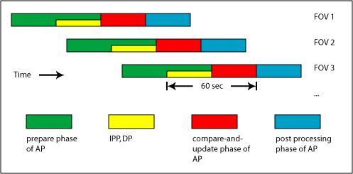
In this diagram, processing of a FOV starts right after observation with the image processing pipeline (IPP) which is followed by the DP, and finally the AP. The yellow and red boxes together represent processing which must happen in the 60 second window. Please note the boxes are not drawn to scale - IPP and DP are likely to take up more of the 60 second window than the diagram suggests. Also note that interaction with the moving object pipeline (MOPS) is omitted, but that there is some planned interaction between it and the AP (notably when a DIA source is mis-classified as an object rather than a moving object).
The database tests are currently focused on how to partition Object and DIASource such that the prepare phase is as fast as possible, and on how to perform the distance based crossmatch of the compare-and-update phase. Tests of database updates, inserts, and of how quickly such changes can be moved from in-memory tables to disk based tables will follow at a later date.
The tests are currently being performed using the USNO-B catalog as a stand-in for the Object table. USNO-B contains 1045175763 objects, so is a bit less than half way to satisfying the DC2 requirement of simulating LSST operations at 10% scale for DR1 (23.09 billion objects).
8.1 Code¶
The code for the tests is available here. The following files are included:
lsstpart/Makefile |
Builds objgen, chunkgen, and bustcache |
lsstpart/bustcache.cpp |
Small program that tries to flush OS file system cache |
lsstpart/chunkgen.cpp |
Generates chunk and stripe descriptions |
lsstpart/crossmatch.sql |
SQL implementation of distance based crossmatch using the zone algorithm [10] |
lsstpart/distribution.sql |
SQL commands to calculate the spatial distribution of the Object table (used to pick test regions and to generate fake Objects) |
lsstpart/genFatObjectFiles.py |
Generates table schemas for “fat” tables |
lsstpart/objgen.cpp |
Program for generating random (optionally perturbed) subsets of tables, as well as random positions according to a given spatial distribution |
lsstpart/prepare.bash |
Loads USNO-B data into Object table |
lsstpart/prepare_chunks.bash |
Creates coarse chunk tables from Object table |
lsstpart/prepare_diasource.bash |
Uses objgen to pick random subsets of Object in the test regions (with perturbed positions). These are used to populate a fake DIASource table |
lsstpart/prepare_fine_chunks.bash |
Loads fine chunk tables from Object |
lsstpart/prepare_stripes.bash |
Loads stripe tables (indexes and clusters on ra) for the test regions from Object |
lsstpart/prepare_zones.bash |
Takes stripe tables generated by prepare_stripes.bash and clusters them on (zoneId, ra) |
lsstpart/prng.cpp |
Pseudo random number generator implementation |
lsstpart/prng.h |
Pseudo random number generator header file |
lsstpart/schema.sql |
Test database schema |
lsstpart/stripe_vars.bash |
Variables used by stripe testing scripts |
lsstpart/test_chunks.bash |
Test script for the coarse chunking approach |
lsstpart/test_fine_chunks.bash |
Test script for the fine chunking approach |
lsstpart/test_funs.bash |
Common test functions |
lsstpart/test_regions.bash |
Ra/dec boundaries for the test FOVs |
lsstpart/test_stripes.bash |
Test script for the stripe approach with ra indexing |
lsstpart/test_zones.bash |
Test script for the stripe approach with (zoneId, ra) indexing |
8.2 Partitioning Approaches¶
8.2.1 Stripes¶
In this approach, each table partition contains Objects having positions falling into a certain declination range. Since a FOV will usually only overlap a small ra range within a particular stripe, indexes are necessary to avoid a table scan of the stripe when reading data into memory.
There are two indexing strategies under consideration here - the first indexes each stripe on ra (and also clusters data on ra). The second indexes and clusters each stripe on (zoneId, ra). In both cases the height of a stripe is 1.75 degrees. The height of a zone is set to 1 arcminute.
8.2.2 Chunks¶
In this approach, a table partition corresponds to an ra/dec box - a
chunk - on the sky. See chunkgen.cpp for details on how chunks are
generated. Basically, the sky is subdivided into stripes of constant
height (in declination), and each stripe is further split into chunks of
constant width (in right ascension). The number of chunks per stripe is
chosen such that the minimum distance between two points in non adjacent
chunks of the same stripe never goes below some limit.
There are no indexes kept for the on-disk tables at all - not even a primary key - so each chunk table is scanned completely when read. Two chunk granularities are tested: the first partitions 1.75 degree stripes into chunks at least 1.75 degrees wide (meaning about 9 chunks must be read in per FOV), the second partitions 0.35 degree stripes into chunks at least 0.35 degrees wide (so about 120 chunks must be examined per FOV).
So with coarse chunks, each logical table (Object, DIASource) is split into 13218 physical tables. With fine chunks, 335482 physical tables are needed. Due to OS filesystem limitations, chunk tables will have to be distributed among multiple databases (this isn’t currently implemented).
8.3 Testing¶
8.3.1 Hardware¶
- SunFire V240
- 2 UltraSPARC IIIi CPUs, 1503 MHz
- 16 GB RAM
- 2 Sun StoreEdge T3 arrays, 470GB each, configured in RAID 5, sustained sequential write speed (256KB blocks) 150 MB/sec, read: 146 MB/sec
- OS: Sun Solaris sun4x_510
- MySQL: version 5.0.27
8.3.2 General Notes¶
Each test is run with both “skinny” objects (USNO-B with some
additions, ~100bytes per row), and “fat” objects (USNO-B plus 200
DOUBLE columns set to random values, ~1.7kB per row) that match the
expected row size (including overhead) of the LSST Object table.
Any particular test is always run twice in a row: this should shed some
light on how OS caching of files affects the results. Between sets of
tests that touch the same tables, the bustcache program is run in an
attempt to flush the operating system caches (it does this by performing
random 1MB reads from the USNO-B data until 16GB of data have been
read).
DIA sources were generated using the objgen program to pick a
random subset of Object in the test FOVs. Approximately 1 in 100
objects were picked for the subset, and each then had its position
perturbed according to a normal distribution with sigma of 2.5e-4
degrees (just under 1 arcsecond).
8.3.3 Test descriptions¶
- Read Object data from the test FOVs into in-memory table(s) with no indexes whatsoever.
- Read Object data from the test FOVs into in-memory table(s)
that have the required indexes created before data is loaded. These
indexes are:
- a primary key on id (hash index) and
- a B-tree index on zoneId for fine chunks, or (for all others) a composite index on (zoneId, ra).
- Read Object data from the test FOVs into in-memory table(s) with no indexes whatsoever, then create indexes (the same ones as above) after loading finishes.
Note that all tests except the fine chunking tests place objects into a single InMemoryObject table (and DIA sources into a single InMemoryDIASource table) which are then used to for cross-matching tests. The fine chunking tests place each on-disk table into a separate in-memory table. This complicates the crossmatch implementation somewhat, but allows for reading many chunk tables in parallel without contention on inserts to a single in-memory table. It allows crossmatch to be parallelized by having different clients call the matching routine for different sub-regions of the FOV (each client is handled by a single thread on the MySQL server).
The following variations on the basic crossmatch are tested (all on in-memory tables):
- Use both match-orders: objects to DIA sources and DIA sources to objects
- Test both slim and wide matching:
- a slim match stores results simply as pairs of keys by which objects and DIA sources can be looked up
- a wide match stores results as a key for a DIA source along with the values of all columns for the matching object. This is important for the fine chunk case, since looking up objects becomes painful when they can be in one of many in-memory tables.
Note that all crossmatches are using a zone-height of 1 arc-minute and a match-radius of 0.000833 degrees (~3 arcseconds).
8.4 Performance Results¶
Crossmatch performance is largely independent of the partitioning approach (there is slight variation since the various approaches don’t necessarily read the same number of objects into memory) except in the fine chunking case where some extra machinery comes into play.
8.4.1 Stripes with ra indexes: Performance Summary¶
For the high density FOV
- 3044468 objects are read into memory
- ? objects read from disk
For the low density FOV
- 76073 objects are read into memory
- ? objects read from disk
For the average density FOV
- 373763 objects are read into memory
- ? objects read from disk
8.4.1.1 Summary¶
Below, elapsed times for multiple runs of every test performed are listed.
| Test | FOV | Row Size | Time - 1st run |
|---|---|---|---|
| Load test | High density | Skinny | 1m1.231s |
| Fat | 5m4.386s | ||
| Low density | Skinny | 0m2.018s | |
| Fat | 0m8.196s | ||
| Avg. density | Skinny | 0m8.067s | |
| Fat | 0m38.553s | ||
| Load and index test | High density | Skinny | 1m30.129s |
| Fat | 5m46.250s | ||
| Low density | Skinny | 0m2.511s | |
| Fat | 0m8.971s | ||
| Avg. density | Skinny | 0m10.991s | |
| Fat | 0m42.360s | ||
| Load then index test | High density | Skinny | 1m50.968s |
| Fat | 14m10.113s | ||
| Low density | Skinny | 0m2.735s | |
| Fat | 0m23.783s | ||
| Avg. density | Skinny | 0m12.012s | |
| Fat | 1m18.091s |
8.4.2 Stripes with (zoneId,ra) indexes: Performance Summary¶
For the high density FOV
- 3044282 objects are read into memory
- note: this is less than the other stripe test (which filters by ra and dec rather than ra and zoneId) due to an off by one error in the zone bounds I was using for the insert query. This slight error doesn’t warrant rerunning the test.
- ? objects read from disk
For the low density FOV
- 76274 objects are read into memory
- ? objects read from disk
For the average density FOV
- 373804 objects are read into memory
- ? objects read from disk
Currently the load test reads in the high density FOV with fat rows in 133 minutes (many times slower than all other approaches). The test is completely IO bound (disk is 80-98% busy, transfer rate is between about 800kB/s and 4MB/s with an average closer to 1MB/s, ~120 r/s sustained). Performance is seek limited - we could attack this problem by putting the indexes for each stripe on separate disks from the data, and furthermore by making sure adjacent stripes don’t share any disk. Due to the extremely poor performance, full test results are omitted. Note also that clustering the stripe tables involved in the test took almost a full week (the tables involved too large for in-memory sorting).
Todo
Setup and test scripts should be double checked for bugs.
8.4.3 Coarse Chunks: Performance¶
For the high density FOV
- 3044468 objects are read into memory
- 5865220 objects read from disk
For the low density FOV
- 76073 objects are read into memory
- ? objects read from disk
For the average density FOV
- 373763 objects are read into memory
- ? objects read from disk
8.4.3.1 Summary¶
Below, elapsed times for multiple runs of every test performed are listed.
| Test | FOV | Row Size | Time - 1st run |
|---|---|---|---|
| Load test | High density | Skinny | 0m36.023s |
| Fat | 4m52.873s | ||
| Low density | Skinny | 0m1.969s | |
| Fat | 0m9.818s | ||
| Avg. density | Skinny | 0m5.517s | |
| Fat | 0m39.668s | ||
| Load and index test | High density | Skinny | 1m0.011s |
| Fat | 5m27.291s | ||
| Low density | Skinny | 0m2.488s | |
| Fat | 0m10.513s | ||
| Avg. density | Skinny | 0m8.013s | |
| Fat | 0m42.883s | ||
| Load then index test | High density | Skinny | 1m14.078s |
| Fat | 13m56.050s | ||
| Low density | Skinny | 0m3.178s | |
| Fat | 0m25.482s | ||
| Avg. density | Skinny | 0m9.924s | |
| Fat | 1m7.057s |
8.4.4 Fine Chunks: Performance¶
For the high density FOV
- 3596852 objects are read into memory
- 3596852 objects read from disk
For the low density FOV
- 105847 objects are read into memory
- 105847 objects read from disk
For the average density FOV
- 446289 objects are read into memory
- 446289 objects read from disk
8.4.4.1 Summary¶
Below, elapsed times for multiple runs of every test performed are listed.
| Test | FOV | Row Size | Time - 1st run |
|---|---|---|---|
| Load test | High density | Skinny | 0m42.217s |
| Fat | 4m50.362s | ||
| Low density | Skinny | 0m3.589s | |
| Fat | 0m22.299s | ||
| Avg. density | Skinny | 0m16.066s | |
| Fat | 0m50.490s | ||
| Load and index test | High density | Skinny | 1m1.573s |
| Fat | 5m19.527s | ||
| Low density | Skinny | 0m4.206s | |
| Fat | 0m24.154s | ||
| Avg. density | Skinny | 0m19.058s | |
| Fat | 0m54.383s | ||
| Load then index test | High density | Skinny | 1m31.118s |
| Fat | 8m8.764s | ||
| Low density | Skinny | 0m5.717s | |
| Fat | 0m52.224s | ||
| Avg. density | Skinny | 0m21.408s | |
| Fat | 1m30.905s |
8.4.5 Crossmatch performance¶
Zone height is 1 arc-minute and match distance is 3 arcseconds for all tests.
A single in-memory table of objects matched against a single in-memory table of DIA sources (and vice versa) :
| FOV | Row size | match-width | match direction | Time - 1st run | Time - 2nd run | Time - 3rd run |
|---|---|---|---|---|---|---|
| High density | Skinny | slim | objects vs. DIA sources | 0m51.989s | 0m52.081s | 0m52.169s |
| DIA sources vs. objects | 0m35.692s | 0m35.371s | 0m35.442s | |||
| wide | objects vs. DIA sources | 0m52.489s | 0m52.498s | 0m52.521s | ||
| DIA sources vs. objects | 0m36.069s | 0m36.180s | 0m35.805s | |||
| Fat | slim | objects vs. DIA sources | 1m4.088s | 1m4.085s | 1m3.906s | |
| DIA sources vs. objects | 0m41.543s | 0m41.763s | 0m41.480s | |||
| wide | objects vs. DIA sources | 1m19.124s | 1m20.902s | 1m11.180s | ||
| DIA sources vs. objects | 0m57.569s | 1m0.377s | 0m48.830s | |||
| Low density | Skinny | slim | objects vs. DIA sources | 0m1.284s | 0m1.278s | 0m1.278s |
| DIA sources vs. objects | 0m0.947s | 0m0.933s | 0m0.945s | |||
| wide | objects vs. DIA sources | 0m1.307s | 0m1.285s | 0m1.283s | ||
| DIA sources vs. objects | 0m0.980s | 0m0.961s | 0m0.950s | |||
| Fat | slim | objects vs. DIA sources | 0m1.582s | 0m1.596s | 0m1.567s | |
| DIA sources vs. objects | 0m1.109s | 0m1.108s | 0m1.104s | |||
| wide | objects vs. DIA sources | 0m1.995s | 0m2.000s | 0m1.883s | ||
| DIA sources vs. objects | 0m1.568s | 0m1.580s | 0m1.459s | |||
| Avg. density | Skinny | slim | objects vs. DIA sources | 0m5.891s | 0m5.887s | 0m5.926s |
| DIA sources vs. objects | 0m4.085s | 0m4.174s | 0m4.148s | |||
| wide | objects vs. DIA sources | 0m5.991s | 0m5.951s | 0m5.939s | ||
| DIA sources vs. objects | 0m4.211s | 0m4.199s | 0m4.161s | |||
| Fat | slim | objects vs. DIA sources | 0m7.392s | 0m7.662s | 0m7.356s | |
| DIA sources vs. objects | 0m4.831s | 0m4.870s | 0m4.871s | |||
| wide | objects vs. DIA sources | 0m9.118s | 0m9.155s | 0m8.587s | ||
| DIA sources vs. objects | 0m6.807s | 0m6.811s | 0m6.234s |
For the fine chunking scheme, the match is processed one stripe at a time (for stripes overlapping the FOV) yielding 11 units of work that are currently executed in serial fashion, but could be run in parallel.
| FOV | Row size | match-width | match direction | Time - 1st run | Time - 2nd run |
|---|---|---|---|---|---|
| High density | Skinny | slim | objects vs. DIA sources | 1m20.287s | 1m20.58s |
| DIA sources vs. objects | 0m56.065s | 0m56.5s | |||
| wide | objects vs. DIA sources | 1m21.169s | 1m21.151s | ||
| DIA sources vs. objects | 0m57.72s | 0m59.873s | |||
| Fat | slim | objects vs. DIA sources | 2m9.347s | 2m9.122s | |
| DIA sources vs. objects | 1m18.949s | 1m18.181s | |||
| wide | objects vs. DIA sources | 2m26.441s | 2m26.048s | ||
| DIA sources vs. objects | 1m37.277s | 1m38.656s | |||
| Low density | Skinny | slim | objects vs. DIA sources | 0m10.592s | 0m10.595s |
| DIA sources vs. objects | 0m8.498s | 0m8.44s | |||
| wide | objects vs. DIA sources | 0m11.056s | 0m11.019s | ||
| DIA sources vs. objects | 0m9.024s | 0m9.228s | |||
| Fat | slim | objects vs. DIA sources | 0m12.064s | 0m12.01s | |
| DIA sources vs. objects | 0m9.141s | 0m9.14s | |||
| wide | objects vs. DIA sources | 0m16.527s | 0m16.656s | ||
| DIA sources vs. objects | 0m13.04s | 0m13.156s | |||
| Avg. density | Skinny | slim | objects vs. DIA sources | 0m15.764s | 0m15.812s |
| DIA sources vs. objects | 0m13.407s | 0m13.378s | |||
| wide | objects vs. DIA sources | 0m16.19s | 0m16.135s | ||
| DIA sources vs. objects | 0m14.016s | 0m14.033s | |||
| Fat | slim | objects vs. DIA sources | 0m21.451s | 0m21.437s | |
| DIA sources vs. objects | 0m16.337s | 0m16.392s | |||
| wide | objects vs. DIA sources | 0m26.95s | 0m26.814s | ||
| DIA sources vs. objects | 0m21.757s | 0m21.92s |
8.4.5.1 Effect of zone height on cross-match performance¶
Varying the zone height doesn’t have a huge effect on performance - smaller zone heights are slightly faster than larger ones, until one reaches 20 arcseconds. At a zone height of 15 arcseconds, performance suddenly drops by a factor of 12 to 16. One possible explanation for this would be that the in-memory zone tables involved in the match pass a size threshold below which table scans are used instead of b-tree range lookups.
8.4.5.1.1 2 arcminute zone height¶
| FOV | Row size | match-width | match direction | Time |
|---|---|---|---|---|
| High density | Skinny | slim | objects vs. DIA sources | 0m54s |
| DIA sources vs. objects | 0m36s | |||
| wide | objects vs. DIA sources | 0m55s | ||
| DIA sources vs. objects | 0m36s |
8.4.5.1.2 45 arcsecond zone height¶
| FOV | Row size | match-width | match direction | Time |
|---|---|---|---|---|
| High density | Skinny | slim | objects vs. DIA sources | 0m51.203s |
| DIA sources vs. objects | 0m34.112s | |||
| wide | objects vs. DIA sources | 0m51.615s | ||
| DIA sources vs. objects | 0m34.511s |
8.4.5.1.3 30 arcsecond zone height¶
| FOV | Row size | match-width | match direction | Time |
|---|---|---|---|---|
| High density | Skinny | slim | objects vs. DIA sources | 0m50.535s |
| DIA sources vs. objects | 0m33.615s | |||
| wide | objects vs. DIA sources | 0m50.989s | ||
| DIA sources vs. objects | 0m34.261s |
8.4.5.1.4 20 arcsecond zone height¶
| FOV | Row size | match-width | match direction | Time |
|---|---|---|---|---|
| High density | Skinny | slim | objects vs. DIA sources | 0m54.990s |
| DIA sources vs. objects | 0m35.113s | |||
| wide | objects vs. DIA sources | 0m55.579s | ||
| DIA sources vs. objects | 0m35.657s |
8.4.5.1.5 15 arcsecond zone height¶
| FOV | Row size | match-width | match direction | Time |
|---|---|---|---|---|
| High density | Skinny | slim | objects vs. DIA sources | 11m18.951s |
| DIA sources vs. objects | 8m25.763s | |||
| wide | objects vs. DIA sources | 11m20.142s | ||
| DIA sources vs. objects | 8m28.906s |
9 Database Performance for Forced Photometry¶
Tested performance of database[♦] using data produced based on SDSS stripe 82 DR8. Database location: lsst10. Test involved running different number of concurrent queries and measuring response time. Each query was selecting sources for a randomly picked bounding box, and returned ~1200-1300 rows. Executed queries looked like:
SELECT scisql_s2CPolyToBin(ra0, decl0, ra1, decl1, ra2, decl2, ra3, decl3) INTO @poly
  FROM Field
  WHERE uniqueId = <uniqueId>;

CALL scisql.scisql_s2CPolyRegion(@poly, 20);

SELECT sourceId, ra, decl, htmId20
  FROM Source AS s
  INNER JOIN scisql.Region AS r ON (s.htmId20 BETWEEN r.htmMin AND r.htmMax)
  WHERE scisql_s2PtInCPoly(ra, decl, @poly) = 1;
First test involved running 10,000 queries total, all on a single node (lsst9) and varying the level of parallelism. During each test all queries were started at exactly the same time, and there was no time delay introduced between them. Results:
| queries per thread | threads | slowest elapsed time [sec] | queries/sec |
|---|---|---|---|
| 10,000 | 1 | 466.2 | 21.5 |
| 5,000 | 2 | 247.7 | 20.2 |
| 2,500 | 4 | 144.4 | 17.3 |
| 2,000 | 5 | 124.2 | 16.1 |
| 1,250 | 8 | 96.6 | 12.9 |
| 1,000 | 10 | 91.8 | 10.9 |
| 400 | 25 | 94.6 | 4.2 |
| 200 | 50 | 95.6 | 1.0 |
| 100 | 100 | 100.0 | 1.0 |
Based on the timer in the test program, the database response time was about the same for each test (~0.2 sec), the limiting factor was threading in the python test program that run all threads.
Second test involved querying the database from two different nodes
(lsst9 and lsst5), 100 threads per node. Measured elapsed time was
comparable to the single-node test:
| queries per thread | threads | slowest elapsed time [sec] | queries/sec |
|---|---|---|---|
| 100 | 50 x 2 machines | 109.0 | 0.9 |
During this test, average query response time was up (approaching ~0.4
sec) - less time was spent in the python client, but the server response
was slower. The limiting factor was server CPU. The server was
completely cpu bound - all 24 cpus were 100% busy. show processlist
showed 200 simultaneous queries processed by the server.
During all these tests there was almost no disk I/O activity. This is
not unexpected, as the entire data set including indexes is < 8 GB in
size, much smaller than RAM available on lsst10.
Related code: see git repo: contrib/forcedPhotDbDemo.git
9.1 About Data Ingest¶
Counts: ~200 million sources (~6GB + 2GB index), ~200K fields (~15 MB).
Loading the data took: ~35 min, sorting by htmId another 35 min.
9.2 Conclusions¶
The server server seems to be handling well 100-200 requests coming in simultaneously, and deliver results in well under a second, even under heavy load, provided there are no other activities competing for mysqld server time and memory. Ideally, it’d be useful to try querying from many more clients, but given in practice forced photometry code will crunch on the data for ~10 sec, thus there there will be ~10 sec delay between queries incoming from the same process, the load seen by the server should be much lower than that tested.
10 References¶
| [1] | [Document-5356]. Tim Axelrod, Robyn Allsman, Jeff Kantor, Jon Myers, Francesco Pierfederici, Serge Monkewicz, Greg Daues, David Gehrig, Steve Pietrowicz, Raymond Plante, Jacek Becla, Kian-Tat Lim, Andrew Becker, Lynne Jones, Russell Owen, Nicole Silvestri, Robert H. Lupton, Jeff Bartels, Phil Pinto, Jeff Kantor, Michael Strauss, and Don Sweeney. LSST Data Challenge 2. 2008. URL, https://ls.st/Document-5356. |
| [2] | [LDM-17]. Tim Axelrod and others. Lsst data challenge 3a final report. 2009. URL, https://ls.st/LDM-17. |
| [3] | [DMTR-12]. Jacek Becla. Qserv 300 node test. 2013. URL, https://ls.st/DMTR-12. |
| [4] | [Document-11625]. Jacek Becla, K-T Lim, and Daniel Wang. Database Architecture. 2011. URL, https://ls.st/Document-11625. |
| [5] | (1, 2) [Document-26276]. Jacek Becla, K-T Lim, and Daniel Wang. Scalable partitioning. 2013. URL, https://ls.st/Document-26276. |
| [6] | [DMTR-21]. Jacek Becla, K-T Lim, and Daniel Wang. Early (pre-2013) Large-Scale Qserv Tests. 2013. URL, https://ls.st/DMTR-21. |
| [7] | [LDM-141]. Jacek Becla and K.-T. Lim. Data management storage sizing and i/o model. 2013. URL, https://ls.st/LDM-141. |
| [8] | (1, 2) [Document-11701]. Jacek Becla, Kian-Tat Lim, and Daniel Wang. Evaluation of solid state disks. 2011. URL, https://ls.st/Document-11701. |
| [9] | [LDM-135]. Jacek Becla, Daniel Wang, Serge Monkewitz, K-T Lim, Douglas Smith, and Bill Chickering. Database design. 2013. URL, https://ls.st/LDM-135. |
| [10] | Jim Gray. The zones algorithm for finding points-near-a-point or cross-matching spatial datasets. Technical Report MSR-TR-2006-52, Microsoft, April 2006. URL: https://www.microsoft.com/en-us/research/publication/the-zones-algorithm-for-finding-points-near-a-point-or-cross-matching-spatial-datasets/. |
| [11] | (1, 2, 3) [Document-9044]. Jeff Kantor, Tim Axelrod, Robyn Allsman, Mike Freemon, and K-T Lim. Data Challenge 3b Overview. 2010. URL, https://ls.st/Document-9044. |
| [12] | [LDM-552]. Fritz Mueller. Qserv software test specification. 2017. URL, https://ls.st/LDM-552. |
| [13] | [Document-9541]. Ray Plante, Robyn Allsman, Tim Axelrood, Jacek Becla, Cristina Beldica, Greg Daues, Jeff Kantor, Jonathan Myers, Russell Owen, and Steve Pietrowicz. Results from data challenge 1. 2010. URL, https://ls.st/Document-9541. |
| [14] | L. Nicastro and G. Calderone. Indexing Astronomical Database Tables using HTM and HEALPix. In R. W. Argyle, P. S. Bunclark, and J. R. Lewis, editors, Astronomical Data Analysis Software and Systems XVII, volume 394 of Astronomical Society of the Pacific Conference Series, 487. August 2008. arXiv:0711.4964. |
| [*] | It is worth noting that in real production we do not anticipate to manage billion+ rows in a single physical table - the Qserv system that we are developing will split every large table into smaller, manageable pieces. |
| [†] | Some of these optimizations will not be required when we use Qserv, as Qserv will apply them internally. |
| [‡] | Original location of this report: https://dev.lsstcorp.org/trac/wiki/db/SpatialJoinPerf |
| [§] | Original location of this 2009 report: https://dev.lsstcorp.org/trac/wiki/db/BuildSubPart |
| [¶] | Original location of this 2009 report: https://dev.lsstcorp.org/trac/wiki/db/SubPartOverhead |
| [#] | Original location of this 2009 report: https://dev.lsstcorp.org/trac/wiki/MyIsamCompression |
| [♠] | Original location of this 2009 report: https://dev.lsstcorp.org/trac/wiki/DbStoringRefCat |
| [♥] | Original location of this 2007 report: https://dev.lsstcorp.org/trac/wiki/db/DC2/PartitioningTests |
| [♦] | Original location of this 2012 report: https://dev.lsstcorp.org/trac/wiki/db/tests/ForcedPhoto |